

Appendix 1
Cohort Component Population Model
The model [14] was run over a 5-year time-step and alternated using observed values in census years (effectively resetting the "projections" model) and calculated values stored from the previous step as seed for inter-decadal years. The birth and death rates for census years were used as is and in inter-decadal years were created from an average of the bordering observed census years. Again, the state rates were applied to each municipality individually with no regards to sex or race composition. This application of state rates onto individual municipalities may introduce error in the output of the model if each area has significantly different birth and death rates [15] . The model is shown in Equation 1 where t is time, Pi is the population of a single age group, Bi is births for that age group, Ai is the number of people aging out of the group and Di is the number of deaths for that group. Note that Ai-1 is the number of people aging out of the younger age group and moving up.
)
Equation 1
Age groups were comprised of five-year increments starting at 0-4 and ending at 85+. Migration was set to zero as rates for entering and leaving the state were unavailable and the results were then compared to the observed numbers. The difference between these two sets of numbers is then attributed to migration. This is a similar method to what Kenneth Johnson has used to determine migration rates between counties. (Johnson 2000) The model was run on each individual municipality and the state as a whole to represent a baseline for comparison. This method yielded results only for the decades of the 1970's and 1980's and not the 1990's since the 2000 census numbers were unavailable at the time of this research.
Age Structure Deviation Analysis
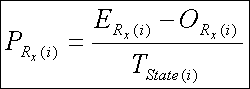
Age Structure Deviation Analysis relies upon taking the overall non-age group specific totals to each region (i.e.; urban and non-urban) in the state and creating a factor representing the proportion of the state's total population that lived in that region (See Equation 2 ). For example, if 60% of the state's total population lived in the urban areas and 40% of the state's total population lived in the non-urban areas then the factors would be 0.60 and 0.40 respectively. The factor is then multiplied against the state total for each age group (0-4, 5-9, etc...) and the result is the expected number of people, in that age group, that should exist in that region, assuming that the age structure of the region and the state are the same (See Equation 3 ). Any deviation between the value computed and the observed value is the number of people not in the region but should be if the age structures were the same [16] (See Equation 4 ). This value is assumed to be an age specific residential preference. The value is then made relative, to adjust for the age structure effect, by dividing by the total number of people in that age group in the state (See Equation 5 ).
)
)
)
)
If a similar pattern of age specific preference occurs year after year, then there must be a pattern of migration occurring internally in the state in order for this to occur. Therefore, in the absence of age specific migration rates between the two regions, evidence of migration (in net terms) can still be found based on the effect it has on the age structure of the population, providing there is an age specific preference for housing.
Equations:
Equation 2
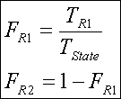 |
Where F is the factor and T is the total number of people in the region (R) denoted by the subscript.
Equation 3
Where E is the expected number of people in the region (Rx) and age group (i) denoted by the subscript.
Equation 4
Where O is the observed number of people in the region and age group denoted by the subscript and N is the difference between expected and observed values.
Adjusting for the uneven age structure by dividing the result by the total number of people in the state belonging in that age group to yield P. P is the percentage of people preferring one area to another.
Equation 5
 |
Thomas Bolioli